brute force attempt to understand RNN
As of today, it’s not feasible to fully understand LLM. Therefore, scientists are hypothesizing that studying a toy model would help us to understand the big model. I came across such toy model released by ARC and I tried to understand their understanding.
As an Mechanistic Interpretability enthusiast, I were curious to study the model by myself and it’s an attempt to explain the understanding in my words and I also think it’s beneficial to have multiple explanation for same thing.
Problem Setup
ARC released multiple toy model, trained to do different algorithmic task. However, I chose a model named argmax2 which is trained to predict the second highest number from the input sequence. eg: 3 is the second largest number among the input sequence [3,4]. It is an RNN based model with different parameter size. But we chose the one with 2 hidden size and 2 input sequence to start with.
def forward(self, x, init_state=None):
    batch_size = x.shape[0]
    if init_state is None:
        # initial hidden state set to zero
        h = x.new_zeros(batch_size, self.hidden_size)
    else:
        h = init_state
    for t in range(x.shape[1]):
        xt = x[:, t : t + 1]
        # shape of i2h and h2h are: (2,1) and (2,2)
        h = th.nn.functional.relu(self.i2h(xt) + self.h2h(h))
    # shape of output: (2,2)
    return self.output(h)
The chosen argmax2 model returns two neuron and the neuron with the highest value is the position of second highest number among the inputs. The below example takes [3,4] as input and return [0.4,0.1] since 3 is the second highest number.
We asked ourself a question; What makes the \(output_{00}> output_{10}\). It’s obvious that answering the question would answer how model works
Sheer Brute Force
To answer the question, we must know what’s going inside the model. RNN calculates hidden state for each time step. the hidden state is calculated based on the current input entry and the previous hidden state, with number of time step decided by the length of the sequence.
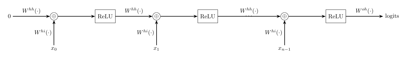
In our model, there are two entries in the input sequence so we calculate two hidden state to uncover the working of the model.
Hidden state 1:
\[h_1 = ReLU(W_{hh}.h_0 + W_{hi}.{x_0}); W_{hi} = \begin{bmatrix} hi_{00} \\ -hi_{01} \end{bmatrix}\]Here \(h_0 = 0\), since there is no previous hidden state for the current step.
\[h_1 = ReLU(\begin{bmatrix} x_0.hi_{00} \\ -x_0.hi_{01} \end{bmatrix}); \text{ where } ReLU(x) = max(0,x)\] \[h_1 = \begin{cases} \begin{bmatrix} x_0.hi_{00} \\ 0 \end{bmatrix} \text{ ; } x_0> 0 \\ \begin{bmatrix} 0 \\ x_0.hi_{01} \end{bmatrix} \text{ ; } x_0< 0 \end{cases}\]The first neuron is activated when \(x_0 >0\) and second neuron is activated when \(x_0<0\), while the other neuron of the each case are zero. \(h_1\) itself is not giving us any valuable information. However, we can infer that ReLu converting the function into piecewise function based on the signs of the input.
Hidden state 2:
We have directly jumped to result of \(h_2\) without showing the intermediate steps. Including those intermediate step would make this post unnecessarily long without adding any substance. The detailed steps are in my notes, please check that if that is of your interest. Here, two cases in \(h_1\) further branched into six cases when deriving \(h_2\). It is sufficient to discuss only the two cases from those six cases to explain the entire model. Since other cases also express similar behavior.
\[h_2 = \begin{cases} \begin{bmatrix} 0 \\ -1.48.x_1 + 2.09.x_0 \end{bmatrix} \text{ ; } x_0 > 0 \text{ ; } 0.7.x_1 < 2.x_1 < x_0 \\ \begin{bmatrix} 1.61.x_1 - 0.58..x_0 \\ -1.48.x_1 + 2.09.x_0 \end{bmatrix} \text{ ; } x_0 > 0 \text{ ; } 0.7.x_1 < x_0 < 2.x_1 \\ \text{ ... } \\ \text{ ... } \\ \text{ ... } \end{cases}\]First case:
I plotted the first case to analyze it visually and It unfolded series of insights on itself:
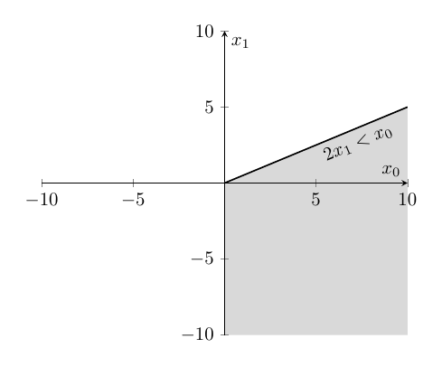
- first case of \(h_2\) carved a region in first quadrant and the entire fourth quadrant.
- \(x_0\) is always greater than \(x_1\) for all the coordinates belongs to that region. try to pick a coordinate in the shaded region and see for yourself.
- in \(h_2\), the second neuron is active, while the first neuron is inactive.
We can conclude that model is trying to learn region where it can tell, \(x_0\) is always greater/lesser than \(x_1\) But, this technique could only work when anyone of the neuron is in active state and the other neuron is in inactive state. Therefore, we’ll analyze the second case where both the neurons are active.
Second case:
The second case of the piecewise function spans the region in first quadrant, around the line \(x_0=x_1\).
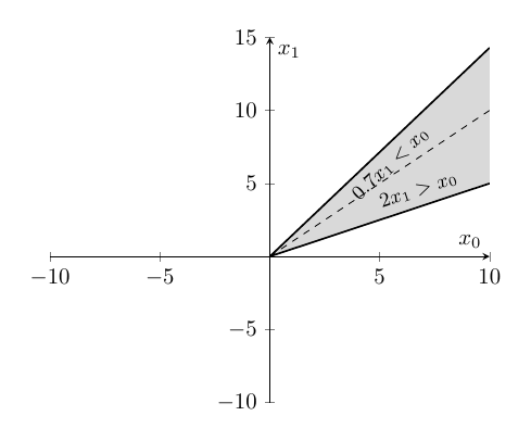
It also worth to note that, \(x_0\) is always lesser than \(x_1\) in any of the coordinates above the line \(x_0=x_1\). Conversely, in the other side of the line \(x_0=x_1\), \(x_0\) is always greater than \(x_1\). So, let’s plug the coordinates from both side to gain insights about this case:
- coordinate above the line \(x_0=x_1\):
- coordinate below the line \(x_0=x_1\):
If the output of the different coordinate sparked any insight in you, then you are in the right track. In then second case of \(h_2\), first neuron is always greater than second neuron when \(x_0>x_1\) and inversely when \(x_0<x_1\).
Conclusion
From the discussed cases of \(h_2\), we can say that model is dividing the space into the region, where it can say which of the entry is greater/smaller among the input sequence. I did this experiment to deeply understand the method which was described in the post by the ARC. As I invested more time on this, I was intrigued by several questions and each of the question itself a separate research direction. I’m glad that I did this experiment and also feeling thankful to the ARC team for releasing the toy model. Otherwise, I wouldn’t have had opportunity to work on this experiment. The current brute force method will not work for slightly bigger model. Next, I’m on to learn other mathematical tools like torus to study bigger models!!