Simplest backpropagation explainer without chain rule

Neural Networks learn to predict by backpropagation. This article aims to help you, build a solid intuition about the concept using a simple example. The ideas we learn here can be expanded for bigger nerual network. I assume that you already know how feed forward neural network works.

Before reading the article further, take a pen and paper. The calculation used in this article can be done in the head. But I still want you to do by hand.

“Mathematics is not a spectator sport.” — George Pólya

Calculus: The Art of Change :

Derivation is used throughout the backpropogation, so it’s crucial for us to revise calculus before reaching our desired goal. As title suggests, derivation is used to find how change in value of an variable affect the result. In the context of neural network, how change in weights affects the results of neural networks.

Let’s look at a simple equation:

\[ y = x^3 \]

If we plug in \(x = 2\), we get:

\[ y = 2^3 = 8 \]

Now, what happens if we slightly increase \(x\) by \(0.01\)? Instead of calculating everything again, we can use the derivative.

The derivative of \(y\) is:

\[ \frac{dy}{dx} = 3x^2 \]\[ dy = 3x^2 \times dx \]

Substituting \(x = 2\) and \(dx = 0.01\):

\[ dy = 3(2)^2 \times 0.01 = 12 \times 0.01 = 0.12 \]

So, if \(x\) increases by \(0.01\), \(y\) should increase by about \(0.12\) which is \(8.12\).

Let’s check it:

• At \(x = 2\), \(y = 8\).
• At \(x = 2.01\), plugging into the original equation:

\[ y = (2.01)^3 = 8.120601 \]

The actual change is about \(8.1206\), which is very close to our estimate of \(8.12\).

Note: The derivative is a good approximation function for small changes, does not work well with bigger number. Curious?? plug in \(dx = 0.5\) and see yourself.

No hidden layer

It almost took two days for me to understand backpropagation clearly. The idea finally clicked when I removed the hidden layer and made it a simple one-to-one network. We’ll take the same route to build up intuition, and later we can stack hidden layers to play with multiple weights.

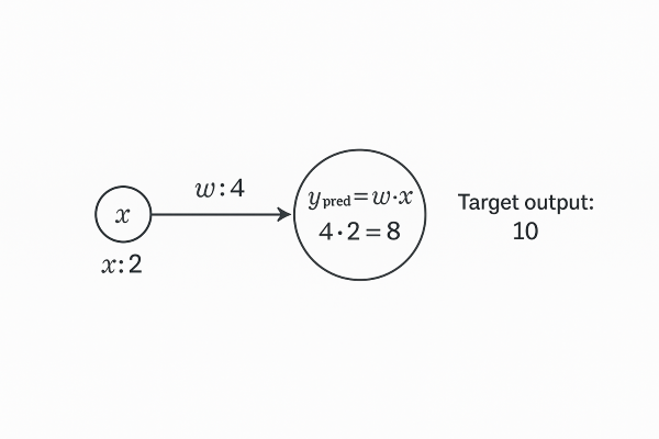
For this simple network, we’ll consider the following parameters:

• Input \( x = 2 \)

• Weight \( w = 4 \)

• Target output \( y = 10 \)

The prediction formula is:

\[ \hat{y} = x \times w \]

Substituting the values:

\[ \hat{y} = 2 \times 4 = 8 \]

Let’s define a cost function to determine the error rate:

\[ \text{Cost} = \hat{y} - y = (x \times w) - 10 \]

\[ \text{Cost} = (2 \times 4) - 10 = 8 - 10 = -2 \]

When the cost approaches zero, the predicted output correlates closely with the target output. But in our case, we are off by 2 units.

How do we decrease the cost?

To reduce the cost, we need to tweak the weight parameter. However, randomly adjusting weights won’t help — it would be like searching for a needle in a haystack. Instead, we use the derivative to understand how the weight affects the cost.

\[ \frac{dC}{dw} = x = 2 \]

The derivative tells us that any change in the weight will change the cost by twice that amount. In other words, if we increase the weight by 1 unit, the cost will change by 2 units.

Since our current cost is negative, it signals that the weight should be increased.(If the cost were positive, we would need to decrease the weight.) Thus, we increase the weight to \( w = 5 \) to move the cost toward zero.

With a Hidden Layer

Let’s add a hidden layer to the same simple network:

• Input \( x = 2 \)
• Weight \( w_1 = 4 \)
• Weight \( w_2 = 3 \)
• Target output \( y_{\text{target}} = 10 \)

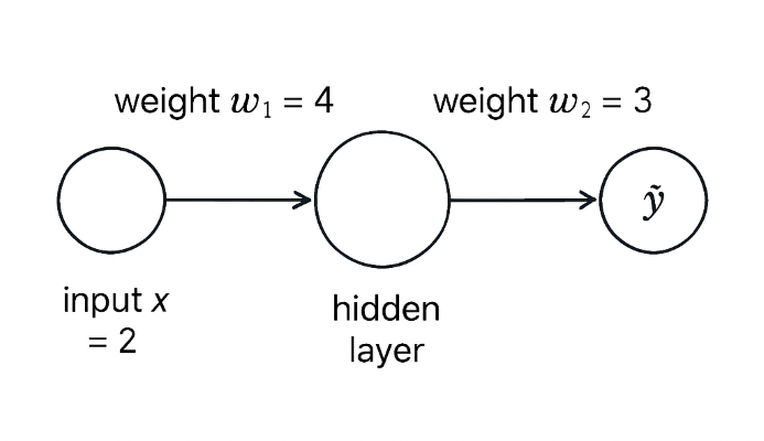
The prediction is given by:

\[ \hat{y} = (x \cdot w_1) \cdot w_2 \]

Substituting the values:

\[ \hat{y} = (2 \times 4) \times 3 = 24 \]

The cost is the difference between the prediction and the target:

\[ \text{Cost} = \hat{y} - y_{\text{target}} = (x \cdot w_1) \cdot w_2 - 10 = 24 - 10 = 14 \]

Now, let’s compute the derivatives:

\[ \frac{dC}{dw_1} = x \cdot w_2 = 2 \times 3 = 6 \]

\[ \frac{dC}{dw_2} = x \cdot w_1 = 2 \times 4 = 8 \]

The derivatives tell us that the \(w_2\) influences the network more than the \(w_1\).

Now, I want you to pause reading and try this quick exercise:

• Increase \( w_1 \) by 0.1 and observe how much \( \hat{y} \) changes.
• Increase \( w_2 \) by 0.1 and observe how much \( \hat{y} \) changes.
• Verify that changing \( w_2 \) causes a bigger change in the output than changing \( w_1 \).

How Do Computers Adjust Weights?

In our first simple network, we manually found the correct weight using our intelligence.
However, computers work much more rudimentary — they adjust the weights using the corresponding derivatives.

The idea is simple:

• Weights with higher influence (higher derivative) are adjusted more.
• Weights with lower influence are adjusted less.

But here’s the catch:
If the derivative values are large, the weights can change abruptly — causing the cost to fluctuate wildly.
This phenomenon is known as the exploding gradient problem.

To prevent this, we multiply the derivative by a small number called the learning rate (e.g., \( 0.01 \)) to ensure smoother learning:

\[ w_1 = w_1 - \text{learning_rate} \times \frac{dC}{dw_1} \]

\[ w_2 = w_2 - \text{learning_rate} \times \frac{dC}{dw_2} \]

By training the model over a large number of samples, the weights are gradually smoothened toward their optimal values, leading to better predictions.

Last Words

I’ve intentionally avoided the chain rule to wrap the core idea in our head. There are a lot of examples out in the wild that use chain rule. Here, is one of my personal favorite